`svgdigitizer.electrochemistry.cv`

This module contains specific functions to digitize cyclic voltammograms. Cyclic voltammograms represent current-voltage curves, where the voltage applied at an electrochemical working electrode is modulated by a triangular wave potential (applied vs. a known reference potential). An example is shown in the top part of the following Figure.

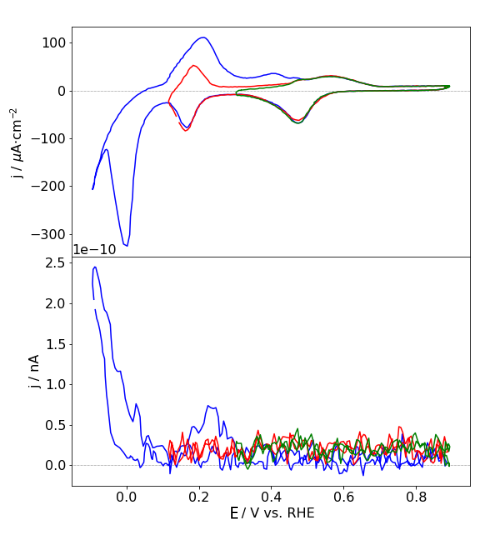
These curves were recorded with a constant scan rate given in units of V / s. This quantity is usually provided in the scientific publication. With this information the time axis can be reconstructed.

The CV can be digitized by importing the plot in an SVG editor, such as Inkscape, where the curve is traced, the axes are labeled and the scan rate is provided. This SVG file can then be analyzed by this class to produce the coordinates corresponding to the original measured values.

A more detailed description on preparing the SVG files is provided in the description of CV or the documentation to create files for echemdb.

For the documentation below, the path of a CV is presented simply as a line.

class svgdigitizer.electrochemistry.cv.CV(svgplot, metadata=None, measurement_type='CV', force_si_units=False)

A digitized cyclic voltammogram (CV) derived from an SVG file, which provides access to the objects of the CV.

Typically, the SVG input has been created by tracing a CV from a publication with a <path> in an SVG editor such as Inkscape. Such a path can then be analyzed by this class to produce the coordinates corresponding to the original measured values.

A detailed description can also be found in the documentation to create files for echemdb.

EXAMPLES:

An instance of this class can be created from a specially prepared SVG file. It requires:

that the x-axis is labeled with U or E (V) and the y-axis

is labeled by I (A) or j (A / cm2)
that the label of the second point (furthest from the origin)

on the x- or y-axis contains a value and a unit

such as <text>j2: 1 mA / cm2</text> or <text>E2: 1 mV</text>.

Optionally, the text of the E/U scale also indicates the

reference scale, e.g., <text>E2: 1 mV vs. RHE</text> for RHE scale.
that a scan rate is provided in a text field such as

<text">scan rate: 50 mV / s</text>, placed anywhere in the SVG file.

In addition the following text fields are accessible with this class

A comment describing the data, i.e.,

<text>comment: noisy data</text>
Other measurements linked to this measurement or performed simultaneously, i.e.,

<text>linked: SXRD, DEMS</text>
A list of tags describing the content of a plot, i.e.,

<text>tags: BCV, HER, OER</text>
The figure label provided in the original plot, i.e.,

<text>figure: 1b</text>

A sample file looks as follows:

>>> from svgdigitizer.svg import SVG
>>> from svgdigitizer.svgplot import SVGPlot
>>> from svgdigitizer.electrochemistry.cv import CV
>>> from io import StringIO
>>> svg = SVG(StringIO(r'''
... <svg>
...   <g>
...     <path d="M 0 100 L 100 0" />
...     <text x="0" y="0">curve: solid</text>
...   </g>
...   <g>
...     <path d="M 0 200 L 0 100" />
...     <text x="0" y="200">E1: 0 mV vs. RHE</text>
...   </g>
...   <g>
...     <path d="M 100 200 L 100 100" />
...     <text x="100" y="200">E2: 1 mV vs. RHE</text>
...   </g>
...   <g>
...     <path d="M -100 100 L 0 100" />
...     <text x="-100" y="100">j1: 0 uA / cm2</text>
...   </g>
...   <g>
...     <path d="M -100 0 L 0 0" />
...     <text x="-100" y="0">j2: 1 uA / cm2</text>
...   </g>
...   <text x="-200" y="330">scan rate: 50 V/s</text>
...   <text x="-300" y="330">comment: noisy data</text>
...   <text x="-400" y="330">figure: 2b</text>
...   <text x="-400" y="530">linked: SXRD, SHG</text>
...   <text x="-400" y="330">tags: BCV, HER, OER</text>
... </svg>'''))
>>> cv = CV(SVGPlot(svg), force_si_units=True)

The data of the CV can be returned as a dataframe with axis ‘t’, ‘E’ or ‘U’, and ‘I’ (current) or ‘j’ (current density). The dimensions are in SI units ‘s’, ‘V’ and ‘A’ or ‘A / m2’.:

>>> cv.df
         t      E     j
0  0.00000  0.000  0.00
1  0.00002  0.001  0.01

The data of this dataframe can also be visualized in a plot, where the axis labels and the data are provided in SI units (not in the dimensions of the original cyclic voltammogram).:

>>> cv.plot()

The properties of the original plot and the dataframe can be returned as a dict:

>>> cv.metadata  == \
... {'experimental': {'tags': ['BCV', 'HER', 'OER']},
...  'source': {'figure': '2b', 'curve': 'solid'},
...  'figure description': {'version': 1,
...                         'type': 'digitized',
...                         'simultaneous measurements': ['SXRD', 'SHG'],
...                         'measurement type': 'CV',
...                         'scan rate': {'value': 50.0, 'unit': 'V / s'},
...                         'fields': [{'name': 'E','unit': 'mV', 'orientation': 'x', 'reference': 'RHE', 'type': 'number'},
...                                    {'name': 'j', 'unit': 'uA / cm2', 'orientation': 'y', 'type': 'number'}],
...                         'comment': 'noisy data'},
...  'data description': {'version': 1,
...                       'type': 'digitized',
...                       'measurement type': 'CV',
...                       'fields': [{'name': 'E', 'type': 'number', 'unit': 'V', 'reference': 'RHE'},
...                                  {'name': 'j', 'type': 'number', 'unit': 'A / m2'},
...                                  {'name': 't', 'type': 'number', 'unit': 's'}]}}
True

property data_schema

A frictionless Schema object, including a Field object describing the data generated with df(). Compared to figure_schema() all fields are given in SI units. A time axis is also included.

EXAMPLES:

>>> from svgdigitizer.svg import SVG
>>> from svgdigitizer.svgplot import SVGPlot
>>> from svgdigitizer.electrochemistry.cv import CV
>>> from io import StringIO
>>> svg = SVG(StringIO(r'''
... <svg>
...   <g>
...     <path d="M 0 100 L 100 0" />
...     <text x="0" y="0">curve: 0</text>
...   </g>
...   <g>
...     <path d="M 0 200 L 0 100" />
...     <text x="0" y="200">E1: 0 V vs. RHE</text>
...   </g>
...   <g>
...     <path d="M 100 200 L 100 100" />
...     <text x="100" y="200">E2: 1 V vs. RHE</text>
...   </g>
...   <g>
...     <path d="M -100 100 L 0 100" />
...     <text x="-100" y="100">j1: 0 uA / cm2</text>
...   </g>
...   <g>
...     <path d="M -100 0 L 0 0" />
...     <text x="-100" y="0">j2: 1 uA / cm2</text>
...   </g>
...   <text x="-200" y="330">scan rate: 50 V/s</text>
... </svg>'''))
>>> cv = CV(SVGPlot(svg), force_si_units=True)
>>> cv.data_schema  
{'fields': [{'name': 'E', 'type': 'number', 'unit': 'V', 'reference': 'RHE'},
            {'name': 'j', 'type': 'number', 'unit': 'A / m2'},
            {'name': 't', 'type': 'number', 'unit': 's'}]}

An SVG with a current axis with dimension I and a voltage axis with dimension U.:

>>> from svgdigitizer.svg import SVG
>>> from svgdigitizer.svgplot import SVGPlot
>>> from svgdigitizer.electrochemistry.cv import CV
>>> from io import StringIO
>>> svg = SVG(StringIO(r'''
... <svg>
...   <g>
...     <path d="M 0 100 L 100 0" />
...     <text x="0" y="0">curve: 0</text>
...   </g>
...   <g>
...     <path d="M 0 200 L 0 100" />
...     <text x="0" y="200">U1: 0 V</text>
...   </g>
...   <g>
...     <path d="M 100 200 L 100 100" />
...     <text x="100" y="200">U2: 1 V</text>
...   </g>
...   <g>
...     <path d="M -100 100 L 0 100" />
...     <text x="-100" y="100">I1: 0 uA</text>
...   </g>
...   <g>
...     <path d="M -100 0 L 0 0" />
...     <text x="-100" y="0">I2: 1 uA</text>
...   </g>
...   <text x="-200" y="330">scan rate: 50 V/s</text>
... </svg>'''))
>>> cv = CV(SVGPlot(svg), force_si_units=True)
>>> cv.data_schema  
{'fields': [{'name': 'U', 'type': 'number', 'unit': 'V', 'reference': 'unknown'},
            {'name': 'I', 'type': 'number', 'unit': 'A'},
            {'name': 't', 'type': 'number', 'unit': 's'}]}

property figure_schema

A frictionless Schema object, including a Fields object describing the voltage and current axis of the original plot including original units. The reference electrode of the potential/voltage axis is also given (if available).

EXAMPLES:

>>> from svgdigitizer.svg import SVG
>>> from svgdigitizer.svgplot import SVGPlot
>>> from svgdigitizer.electrochemistry.cv import CV
>>> from io import StringIO
>>> svg = SVG(StringIO(r'''
... <svg>
...   <g>
...     <path d="M 0 100 L 100 0" />
...     <text x="0" y="0">curve: 0</text>
...   </g>
...   <g>
...     <path d="M 0 200 L 0 100" />
...     <text x="0" y="200">E1: 0 V vs. RHE</text>
...   </g>
...   <g>
...     <path d="M 100 200 L 100 100" />
...     <text x="100" y="200">E2: 1 V vs. RHE</text>
...   </g>
...   <g>
...     <path d="M -100 100 L 0 100" />
...     <text x="-100" y="100">j1: 0 uA / cm2</text>
...   </g>
...   <g>
...     <path d="M -100 0 L 0 0" />
...     <text x="-100" y="0">j2: 1 uA / cm2</text>
...   </g>
...   <text x="-200" y="330">scan rate: 50 V/s</text>
... </svg>'''))
>>> cv = CV(SVGPlot(svg))
>>> cv.figure_schema  
{'fields': [{'name': 'E', 'type': 'number', 'unit': 'V', 'orientation': 'x', 'reference': 'RHE'},
            {'name': 'j', 'type': 'number', 'unit': 'uA / cm2', 'orientation': 'y'}]}

plot()

Visualize the digitized cyclic voltammogram with values in SI units.

EXAMPLES:

>>> from svgdigitizer.svg import SVG
>>> from svgdigitizer.svgplot import SVGPlot
>>> from svgdigitizer.electrochemistry.cv import CV
>>> from io import StringIO
>>> svg = SVG(StringIO(r'''
... <svg>
...   <g>
...     <path d="M 0 100 L 100 0" />
...     <text x="0" y="0">curve: solid</text>
...   </g>
...   <g>
...     <path d="M 0 200 L 0 100" />
...     <text x="0" y="200">E1: 0 mV</text>
...   </g>
...   <g>
...     <path d="M 100 200 L 100 100" />
...     <text x="100" y="200">E2: 1 mV</text>
...   </g>
...   <g>
...     <path d="M -100 100 L 0 100" />
...     <text x="-100" y="100">j1: 0 uA / cm2</text>
...   </g>
...   <g>
...     <path d="M -100 0 L 0 0" />
...     <text x="-100" y="0">j2: 1 uA / cm2</text>
...   </g>
...   <text x="-200" y="330">scan rate: 50 V/s</text>
... </svg>'''))
>>> cv = CV(SVGPlot(svg))
>>> cv.plot()

svgdigitizer.electrochemistry.cv

`svgdigitizer.electrochemistry.cv`