Command Line Interface
The command line interface (CLI) allows creating SVG files from PDFs, which in turn allows digitizing the processed SVG files. Certain plot types have specific commands to recover different kinds of plots with different metadata. All commands and options are revealed with
Note
The preceding ! in the following examples is used to evaluate bash commands in jupyter notebooks. Remove the ! to evaluate the command in the shell.
!svgdigitizer
Usage: svgdigitizer [OPTIONS] COMMAND [ARGS]...

  The svgdigitizer suite.

Options:
  --help  Show this message and exit.

Commands:
  create-svg     Write an SVG that shows `png` or `jpeg` as a linked image.
  cv             Digitize a cylic voltammogram and create a frictionless...
  digitize       Digitize a 2D plot.
  figure         Digitize a figure with units on the axis and create a...
  get-citation   Get the citation from the DOI provided PDF file.
  get-doi        Get the DOI from the provided PDF file.
  paginate       Render PDF pages as individual SVG files with linked PNG...
  plot           Display a plot of the data traced in an SVG.
  rename-by-key  Rename the provided PDF file by the key derived from...
Note
Example files for the use with the svgdigitizer can be found in the repository.
paginate
Create SVG and PNG files from a PDF with
!svgdigitizer paginate --help
Usage: svgdigitizer paginate [OPTIONS] PDF

  Render PDF pages as individual SVG files with linked PNG images.

  The SVG and PNG files are written to the PDF's directory.

Options:
  --pages TEXT          Specify a single page (e.g., '2') or a range (e.g.,
                        '3-5').
  --onlypng             Only produce PNG files.
  --template [basic]    Add builtin template elements in SVG files.
  --template-file FILE  Add template elements from a custom SVG in SVG files.
  --outdir DIRECTORY    Write output files to this directory.
  --doi TEXT            Specify DOI (e.g. '10.1021/ed047p365') if it is not
                        extracted automatically from the PDF file.
  --rename              Specify if files should be named according to the
                        echemdb identifier.
  --help                Show this message and exit.
Example PDFs for testing purposes are available in the svgdigitizer repository.
Examples
Create an SVG with a linked PNG for specific pages in a PDF. Use --pages to select which pages to process.
!svgdigitizer paginate ./files/others/example_plot_paginate.pdf --pages 0
Usage: svgdigitizer paginate [OPTIONS] PDF
Try 'svgdigitizer paginate --help' for help.

Error: Invalid value: Invalid range. Page numbers must be within 1-1.
Download the resulting SVG (example_plot_paginate_p0.svg).
create-svg
Create an SVG with a linked PNG or JPEG from such a file.
!svgdigitizer create-svg --help
Usage: svgdigitizer create-svg [OPTIONS] IMG

  Write an SVG that shows `png` or `jpeg` as a linked image.

Options:
  --template TEXT       Add builtin template elements in SVG files.
  --template-file FILE  Add template elements from a custom SVG in the SVG
                        file.
  --outdir DIRECTORY    Write output files to this directory.
  --help                Show this message and exit.
A Example PNG for testing purposes is available in the svgdigitizer repository.
In addition to the linked image, elements for annotating a curve in a figure
can be embedded in the SVG from builtin templates with the --template option.
!svgdigitizer paginate ./files/others/example_plot_paginate.pdf --pages 1 --template basic
Custom templates can be included by providing to the --template-file argument a custom SVG <file path>.
Only elements of the template SVG residing inside a group/layer with the id attribute digitization-layer are imported.
!svgdigitizer paginate ./files/others/example_plot_paginate.pdf --pages 1 --template-file ./files/others/custom_template.svg
digitize
Produces a CSV from the curve traced in the SVG.
!svgdigitizer digitize --help
Usage: svgdigitizer digitize [OPTIONS] SVG

  Digitize a 2D plot.

  Produces a CSV from the curve traced in the SVG.

Options:
  --sampling-interval FLOAT  Sampling interval on the x-axis with respect to
                             the x-axis values.
  --outdir DIRECTORY         Write output files to this directory.
  --skewed                   Detect non-orthogonal skewed axes going through
                             the markers instead of assuming that axes are
                             perfectly horizontal and vertical.
  --help                     Show this message and exit.
Examples
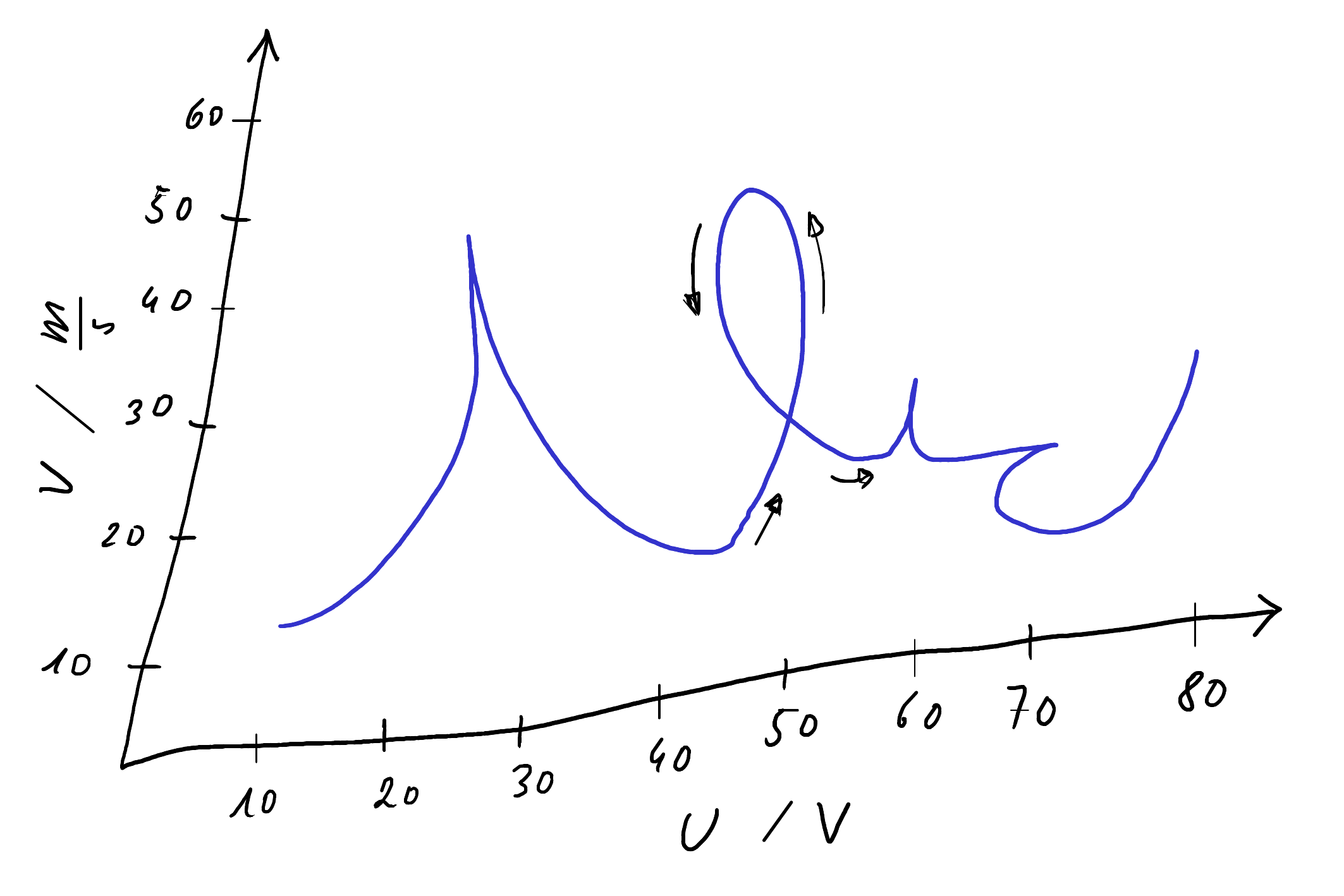
Consider the following skewed plot.

An unskewed digitized CSV can be created with
!svgdigitizer digitize ./files/others/example_plot_p0_demo_digitize.svg --skewed
The CSV can, for example, be imported as a pandas dataframe to create a plot.
import pandas as pd

df = pd.read_csv('./files/others/example_plot_p0_demo_digitize.csv')
df.plot(x='U', y='v', ylabel='v')
<Axes: xlabel='U', ylabel='v'>
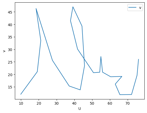
The resulting plot indicates that only the nodes of the spline were connected. To improve the tracing use the --sampling-interval option.
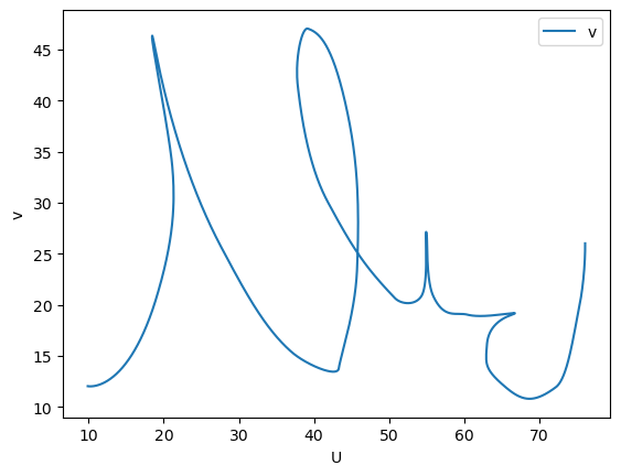
!svgdigitizer digitize ./files/others/example_plot_p0_demo_digitize.svg --skewed --sampling-interval 0.01
The result looks as follows
<Axes: xlabel='U', ylabel='v'>
Note
The use of svgdigitizer digitize is discouraged when your axis labels contain units, because the output CSV does not contain this information. Use svgdigitizer figure instead, which creates a frictionless datapackage (CSV + JSON).
plot
Display a plot of the data traced in an SVG
!svgdigitizer plot --help
Usage: svgdigitizer plot [OPTIONS] SVG

  Display a plot of the data traced in an SVG.

Options:
  --sampling-interval FLOAT  Sampling interval on the x-axis with respect to
                             the x-axis values.
  --skewed                   Detect non-orthogonal skewed axes going through
                             the markers instead of assuming that axes are
                             perfectly horizontal and vertical.
  --help                     Show this message and exit.
Note
The plot will only be displayed, when your shell is configure accordingly.
Examples
The plot of an annotated example SVG (with skewed axis) with a specific sampling interval can be created with
!svgdigitizer plot ./files/others/example_plot_p0_demo_digitize.svg --skewed --sampling-interval 0.01
figure
The figure command produces a CSV and an JSON with additional metadata, which contains, for example, information on the axis units. In addition it will reconstruct a time axis, when the rate at which the data on the x-axis is given in a text label in the SVG such as scan rate: 30 m/s. Here the unit must be equivalent to that on the x-axis divided by a time.
!svgdigitizer figure --help
Usage: svgdigitizer figure [OPTIONS] SVG

  Digitize a figure with units on the axis and create a frictionless
  datapackage.

  The resulting CVS contains a time axis, when text label with a scan rate is
  given in the SVG whose units must be of type `x-axis unit / time unit`, such
  as `scan rate: 50 K / s`.

Options:
  --sampling-interval FLOAT  Sampling interval on the x-axis with respect to
                             the x-axis values.
  --outdir DIRECTORY         Write output files to this directory.
  --metadata FILENAME        yaml file with metadata
  --si-units                 Convert units of the plot and CSV to SI (only if
                             they are compatible with astropy units).
  --bibliography FILENAME    Adds bibliography data from a bibfile located in
                             a specified directory as descriptor to the
                             datapackage.
  --citation-key TEXT        The citation related to this file, which is
                             included in the bibliography provided with
                             --bibliography.
  --skewed                   Detect non-orthogonal skewed axes going through
                             the markers instead of assuming that axes are
                             perfectly horizontal and vertical.
  --help                     Show this message and exit.
Note
Flags --bibliography, --metadata and si-units are covered in the advanced section section below.
Examples
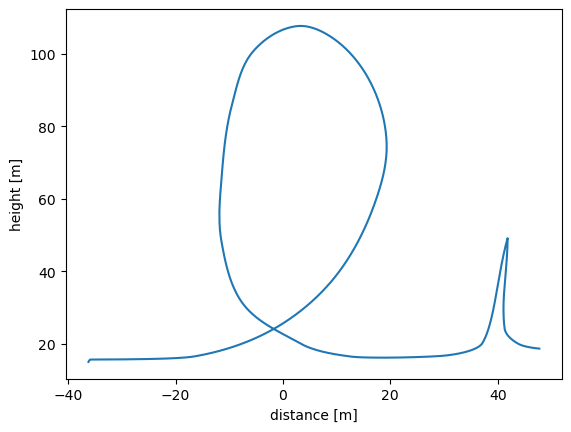
Consider the following figure where the annotated SVG (looping_scan_rate.svg) contains a scan rate.
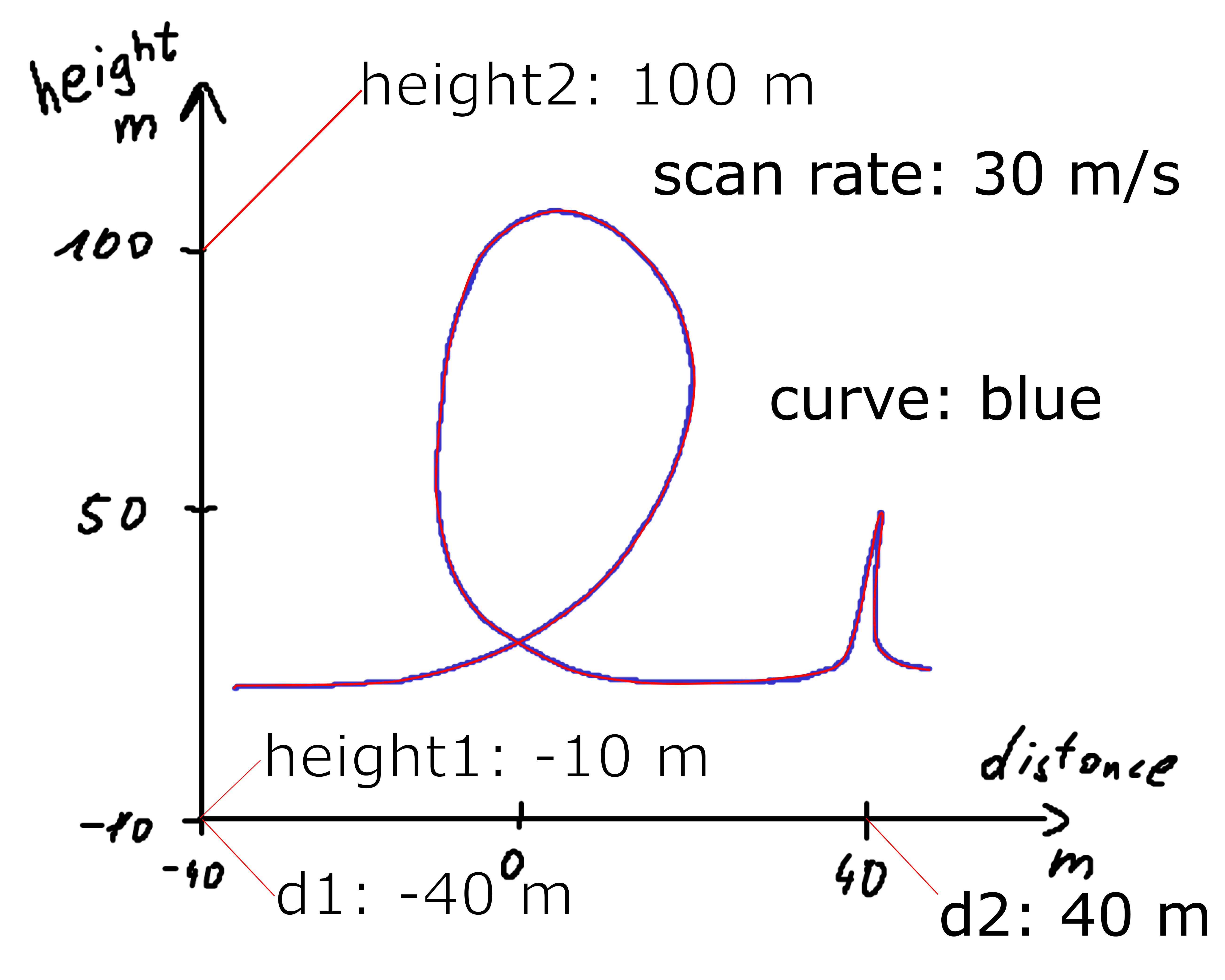
Digitize the figure with
!svgdigitizer figure ./files/others/looping_scan_rate.svg --sampling-interval 0.01
No text with `figure` containing a label such as `figure: 1a` found in the SVG.
Resulting in
<Axes: xlabel='distance [m]', ylabel='height [m]'>
cv
The cv option is designed specifically to digitze cyclic voltammograms (CVs). Overall the command cv has the same functionality as the figure command. The differences are as follows.
Certain keys in the output metadata are directly related to cyclic voltammetry measurements.
The units on the x-axis must be equivalent to volt
Ugiven in units ofVand those on the y-axis equivalent to currentIin units ofAor current densityjin units ofA / m2.The voltage unit can be given vs. a reference, such as
V vs. RHE. In that case, the dimension should beEinstead ofU.The
--sampling-intervalshould be provided in units ofmV.
These standardized CV data are, for example, used in the echemdb database.
!svgdigitizer cv --help
Usage: svgdigitizer cv [OPTIONS] SVG

  Digitize a cylic voltammogram and create a frictionless datapackage.

  The sampling interval should be provided in mV.

  For inclusion in www.echemdb.org.

Options:
  --sampling-interval FLOAT  Sampling interval on the x-axis with respect to
                             the x-axis values.
  --outdir DIRECTORY         Write output files to this directory.
  --metadata FILENAME        YAML file with metadata
  --bibliography FILENAME    Adds bibliography data from a bibfile located in
                             a specified directory as descriptor to the
                             datapackage.
  --citation-key TEXT        The citation related to this file, which is
                             included in the bibliography provided with
                             --bibliography.
  --si-units                 Convert units of the plot and CSV to SI (only if
                             they are compatible with astropy units).
  --skewed                   Detect non-orthogonal skewed axes going through
                             the markers instead of assuming that axes are
                             perfectly horizontal and vertical.
  --help                     Show this message and exit.
Note
Flags --bibliography, --metadata and si-units are covered in the advanced section section below.
Examples
An annotated example SVG is shown in the following figure.
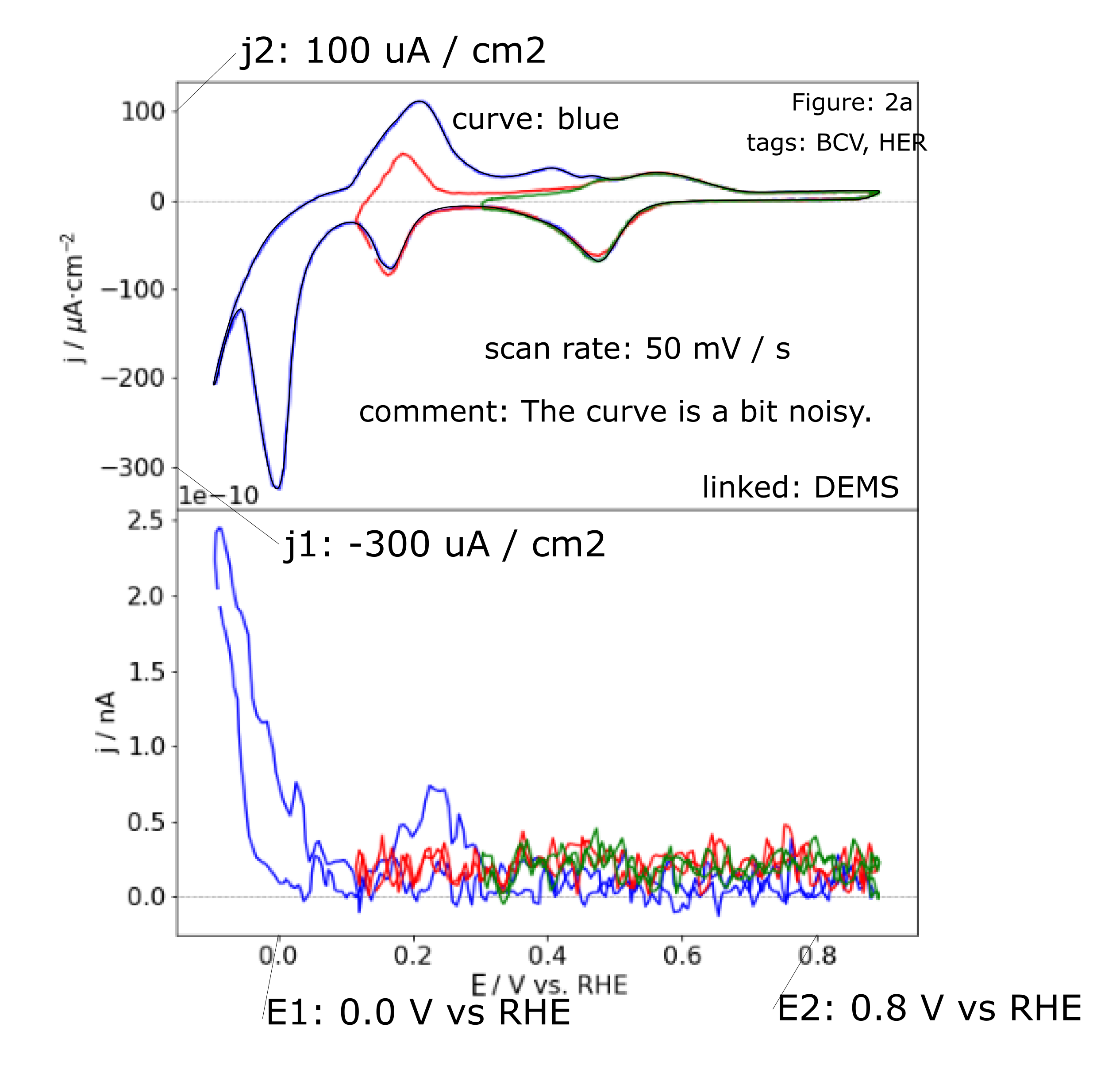
which can be digitzed via
!svgdigitizer cv ./files/mustermann_2021_svgdigitizer_1/mustermann_2021_svgdigitizer_1_f2a_blue.svg --sampling-interval 0.01
Advanced flags
--si-units
The flag --si-unit is used by the figure command and commands that inherit from figure, such as the cv command. The units are converted to SI units, if they are compatible with the astropy unit package. The values in the CSV are scaled respectively and the new units are provided in the output JSON files.
Warning
In some cases conversion to SI units might not result in the desired output. For example, even though V is considered as an SI unit, astropy might convert the unit to W / A or A Ohm.
--metadata
The flag --metadata allows adding metadata to the resource of the datapackage from a yaml file. It is used by the figure command and commands that inherit from figure, such as the cv command.
Consider the following figure where the annotated SVG (looping_scan_rate.svg).
We collect additional metadata in a YAML file (looping_scan_rate_yaml.yaml) describing the underlying “experiment”.
!svgdigitizer figure ./files/others/looping_scan_rate_yaml.svg --metadata ./files/others/looping_scan_rate_yaml.yaml --sampling-interval 0.01
No text with `figure` containing a label such as `figure: 1a` found in the SVG.
The metadata from the YAML is included in the JSON of the resulting datapackage and is accessible with a JSON loader
import json
with open('./files/others/looping_scan_rate_yaml.json', 'r') as f:
    metadata = json.load(f)
metadata
{'resources': [{'name': 'looping_scan_rate_yaml',
   'type': 'table',
   'path': 'looping_scan_rate_yaml.csv',
   'scheme': 'file',
   'format': 'csv',
   'mediatype': 'text/csv',
   'encoding': 'utf-8',
   'schema': {'fields': [{'name': 't', 'type': 'number', 'unit': 's'},
     {'name': 'd', 'type': 'number', 'unit': 'm'},
     {'name': 'height', 'type': 'number', 'unit': 'm'}]},
   'metadata': {'echemdb': {'cyclist': 'John Doe',
     'title': 'Cyclist driving through a looping.',
     'description': 'The cyclist rides at a constant speed of 5 m/s along a track including a looping.',
     'experimental': {'tags': []},
     'source': {'figure': '', 'curve': 'blue'},
     'figureDescription': {'type': 'digitized',
      'simultaneousMeasurements': [],
      'measurementType': 'custom',
      'fields': [{'name': 'd',
        'type': 'number',
        'unit': 'm',
        'orientation': 'horizontal'},
       {'name': 'height',
        'type': 'number',
        'unit': 'm',
        'orientation': 'vertical'}],
      'comment': '',
      'scanRate': {'value': 30.0, 'unit': 'm / s'}}}}}]}
or directly with the frictionless interface
from frictionless import Package
package = Package('./files/others/looping_scan_rate_yaml.json')
package
{'resources': [{'name': 'looping_scan_rate_yaml',
                'type': 'table',
                'path': 'looping_scan_rate_yaml.csv',
                'scheme': 'file',
                'format': 'csv',
                'mediatype': 'text/csv',
                'encoding': 'utf-8',
                'schema': {'fields': [{'name': 't',
                                       'type': 'number',
                                       'unit': 's'},
                                      {'name': 'd',
                                       'type': 'number',
                                       'unit': 'm'},
                                      {'name': 'height',
                                       'type': 'number',
                                       'unit': 'm'}]},
                'metadata': {'echemdb': {'cyclist': 'John Doe',
                                         'title': 'Cyclist driving through a '
                                                  'looping.',
                                         'description': 'The cyclist rides at '
                                                        'a constant speed of 5 '
                                                        'm/s along a track '
                                                        'including a looping.',
                                         'experimental': {'tags': []},
                                         'source': {'figure': '',
                                                    'curve': 'blue'},
                                         'figureDescription': {'type': 'digitized',
                                                               'simultaneousMeasurements': [],
                                                               'measurementType': 'custom',
                                                               'fields': [{'name': 'd',
                                                                           'type': 'number',
                                                                           'unit': 'm',
                                                                           'orientation': 'horizontal'},
                                                                          {'name': 'height',
                                                                           'type': 'number',
                                                                           'unit': 'm',
                                                                           'orientation': 'vertical'}],
                                                               'comment': '',
                                                               'scanRate': {'value': 30.0,
                                                                            'unit': 'm '
                                                                                    '/ '
                                                                                    's'}}}}}]}
For electrochemical data an example YAML can be found here.
--bibliography
The flag --bibliography in combination with --citation-key adds a bibtex bibliography entry to the JSON of the produced datapackage. It is used by the figure command and commands that inherit from figure such as the cv command.
If --citation-key is not provided a key is looked for in the metadata provided in the yaml via --metadata, where it must be stored in source.citationKey
Requirements:
a BIB file containing BibTex styled citations such as in the
here.a valid key that can be found in the BibTex file.
(optional) the
YAML filefile must contain a citationKey to the bib file such as
source:
  citationKey: BIB_FILENAME  # without file extension
!svgdigitizer figure ./files/others/looping_scan_rate_bib.svg --bibliography ./files/others/cyclist2023.bib --metadata ./files/others/looping_scan_rate_bib.yaml --sampling-interval 0.01
No text with `figure` containing a label such as `figure: 1a` found in the SVG.
The bib file content is included in the resulting JSON of the datapackge
from frictionless import Package
package = Package('./files/others/looping_scan_rate_bib.json')
package
{'resources': [{'name': 'looping_scan_rate_bib',
                'type': 'table',
                'path': 'looping_scan_rate_bib.csv',
                'scheme': 'file',
                'format': 'csv',
                'mediatype': 'text/csv',
                'encoding': 'utf-8',
                'schema': {'fields': [{'name': 't',
                                       'type': 'number',
                                       'unit': 's'},
                                      {'name': 'd',
                                       'type': 'number',
                                       'unit': 'm'},
                                      {'name': 'height',
                                       'type': 'number',
                                       'unit': 'm'}]},
                'metadata': {'echemdb': {'cyclist': 'John Doe',
                                         'title': 'Cyclist driving through a '
                                                  'looping.',
                                         'description': 'The cyclist rides at '
                                                        'a constant speed of 5 '
                                                        'm/s along a track '
                                                        'including a looping.',
                                         'source': {'citationKey': 'cyclist2023',
                                                    'figure': '',
                                                    'curve': 'blue',
                                                    'bibdata': '@article{cyclist2023,\n'
                                                               '    author = '
                                                               '"Doe, John",\n'
                                                               '    title = '
                                                               '"Cycling a '
                                                               'Looping",\n'
                                                               '    journal = '
                                                               '"New Open '
                                                               'Access '
                                                               'Journal",\n'
                                                               '    volume = '
                                                               '"1",\n'
                                                               '    number = '
                                                               '"1",\n'
                                                               '    pages = '
                                                               '"1--4",\n'
                                                               '    year = '
                                                               '"2023",\n'
                                                               '    publisher '
                                                               '= "Some '
                                                               'publisher"\n'
                                                               '}\n'},
                                         'experimental': {'tags': []},
                                         'figureDescription': {'type': 'digitized',
                                                               'simultaneousMeasurements': [],
                                                               'measurementType': 'custom',
                                                               'fields': [{'name': 'd',
                                                                           'type': 'number',
                                                                           'unit': 'm',
                                                                           'orientation': 'horizontal'},
                                                                          {'name': 'height',
                                                                           'type': 'number',
                                                                           'unit': 'm',
                                                                           'orientation': 'vertical'}],
                                                               'comment': '',
                                                               'scanRate': {'value': 30.0,
                                                                            'unit': 'm '
                                                                                    '/ '
                                                                                    's'}}}}}]}